Overdamped langevin dynamics simulations of grain boundary motion

Abstract

Macroscopic properties of structural materials are strongly dependent on their microstructure. However, the modeling of their evolution is a complex task because of the mechanisms involved such as plasticity, recrystallization, and phase transformations, which are common processes taking place in metallic alloys. This complexity led to a growing interest in atomistic simulations formulated without any auxiliary hypotheses beyond the choice of interatomic potential. In this context, we propose here a model based on an overdamped stochastic evolution of particles interacting through inter-atomic forces. The model settles to the correct thermal equilibrium distribution in canonical and grand-canonical ensembles and is used to study the grain boundary migration. Finally, a comparison of our results with those obtained by molecular dynamics shows that our approach reproduces the complex atomic-scale dynamics of grain boundary migration correctly.

Introduction

The increase in manufacturing of small-scale metallic crystalline materials and their usage in the current nanotechnology era calls for a deeper understanding of their mechanical behavior (Shan et al. 2008; Wang et al. 2014; Chen et al. 2014; Zhang et al. 2017). This can only be achieved by improving our knowledge on the rich physics and complexities at small-scales such as dislocation plasticity, grain boundary (GB) migration, diffusion, phase transformations, and their coupling. To that end, atomistic modeling techniques become more and more relevant not only because they are formulated at the appropriate scale (Mishin et al. 2010) but also they provide information and data for models formulated at mesoscale, e.g., discrete dislocation dynamics (Bulatov et al. 1998; Zepeda-Ruiz et al. 2017), phase field methods (Finel et al. 2010, 2018; Vuppuluri and Vedantam 2016; Salman et al. 2012; Ask et al. 2018) and non-linear elastic models (Minami and Onuki 2007; Salman and Truskinovsky 2011; Geslin et al. 2014; Salman et al. 2019).

Molecular theories postulate the dependence of the energy on the inter-atomic distances and bond angles between pairs of atoms. Afterward, for a given N particle assembly, the evolution of the system is obtained straightforwardly by integrating Newton equations (Rahman 1964). Although it is challenging to obtain interaction potentials that are able to reproduce the thermodynamical properties of a specific material, the major drawback in molecular theories is the limitation on the accessible time and length scales. Typical molecular dynamics (MD) simulations involve approximately 10⁴- 10⁶ atoms (which is equivalent to a few nanometers) and last a time span of a few nanoseconds (Paul 1993). The limitation on the time scale is due to the presence of high phonons frequencies (typically of the order of 10¹² Hz) in crystalline materials that severely restricts the integration time-step.

Several extensions of the original MD have been proposed, such as the Voter’s hyperdynamics (Voter 1997) which provides an accelerated scheme that incorporates directly thermal effects or the Laio and Parrinello’s metadynamics (Laio and Parrinello 2002) which consists in computing free energy barriers. Most of these approaches rely on the transition state theory, which basically consists in treating rare events as Markov processes. Therefore, it has been natural to look at other methods that are directly and fully based on the transition state theory, such as Monte Carlo methods or stochastic overdamped dynamics which do not incorporate inertia and, consequently, automatically exclude lattice vibrations.

Indeed, different methods have been developed in the past to get rid of the time scale associated with phonons and to reach time scales associated with diffusion. More than a decade ago, a continuous atomic-scale method, the phase field crystal method, has been introduced (Elder et al. 2002). It consists in following the evolution of the atomic density, whose maxima correspond to the positions of atoms. The method is attractive as, despite its simplicity, it automatically incorporates elastic effects, multiple crystal orientations and the nucleation and motion of dislocations. Also, as the dynamics is purely dissipative, it gives access (at least in principle) to diffusive time scales. However, being continuous by nature, the numerical implementation requires the use of a grid with grid spacing much smaller than the smallest length scale incorporated in the model, i.e., the atomic size. Therefore, the method is drastically limited to very small system sizes.

Another methodology is based on the fact that, at low enough temperature, diffusion events take place at a small rate and, therefore, these events can be considered as Markov processes. This is at the root of the so-called kinetic Monte Carlo (KMC) method, which consists in following a Markov chain with a catalog of predefined diffusion mechanisms to compute at every time step the escape rate from a local minimum (Bortz et al. 1975; Yip 2005). However, since this catalog is predefined, the system under study has to be discretized and atomic positions are limited to fixed lattice sites. In order to extend KMC to long-range elastic effects and, more importantly, to disordered or distorted configurations (amorphous or liquid state, dislocations, cracks, …), various off-lattice versions have been developed. Among them, we mention the k-ART method, which stands for “kinetic Activation-Relaxation Technique” (El-Mellouhi et al. 2008). This is an off-lattice KMC in which the energy barriers are evaluated “on-the-fly”, which relaxes the need for a predefined catalog. However, the method still relies on a catalog of events which, now, is not predefined but grows along the route of the Markov chain. The updating of this catalog and its use are rather complex (see for example Béland et al. (2011)). For instance, starting from a local minimum, the generation of the transition path associated with a new event requires the random identification of the direction of the lowest local instability and the identification of the subsequent path to the nearest saddle point while the energy is minimized in the hyperplane orthogonal to this direction. All together, these steps require a few hundred (typically 600 to 800 times) evaluations of forces.

The overdamped Langevin method proposed below and the ART KMC belong to the same category, as both rely on Markov dynamics applied to atomic positions. Therefore, they should give access to the same time scales. However, the overdamped Langevin method is much simpler to use, because it does not require the delicate creation and continuous updating of a catalog of events. To our knowledge, this approach, while it is widely used in studying the dynamics in soft matter systems and bio-molecular simulations (Ando et al. 2003; Manghi et al. 2006; Ma et al. 2016a, b) has never been employed in the simulation of crystalline materials.

The aim of this paper is to present a derivation of overdamped Langevin dynamics (LD) equations that reproduce the proper thermal equilibrium distribution in the canonical and grand-canonical ensembles, then to use these equations in the study of temperature- and curvature-driven grain boundary migration.

The paper is organized as follows. First, we describe the overdamped Langevin dynamics and how it can be extended to simulate the grand-canonical thermodynamic ensemble. Also, we give a numerical justification for the application of this overdamped formalism. Finally, we report the results of the application of the LD to the study of grain boundary migration under the sole effect of curvature. The output of the model is then compared with the results obtained by MD. The last section is dedicated to conclusions and perspectives.

Presentation of the model

Overdamped langevin dynamics: general formalism

We first consider the simple situation of the (NVT) thermodynamical ensemble in which the number of particle N, the volume V and the temperature T are fixed. The main objective of the present approach is to avoid the time scale associated with phonons. Therefore, the configurational space in restricted to the coordinates $x_{i}^{n}$, where upper index n=1,...,N refers to a particle and lower index i=1,2,3 to a cartesian coordinate. Correspondingly, the dynamics involves only the first derivatives of $x_{i}^{n}$:

$$ \frac{{dx}_{i}^{n}}{dt} = - \nu^{-1} {\frac {\partial \Phi}{\partial x_{i}^{n}}} + B \eta_{i}^{n}(t), $$

(1)

where $\Phi (\{ x_{i}^{n}\})$ is the potential energy between particles, ν a viscosity coefficient and B the amplitude of a white gaussian noise $\eta _{i}^{n}(t)$ such that $\left \langle \eta _{i}^{n}(t)\right \rangle =0$, $\left \langle \eta _{i}^{n}(t)\eta _{j}^{m}(t^{\prime })\right \rangle =\delta _{nm}\delta _{ij}\delta (t-t^{\prime })$. δ_nm and δ_ij are Kronecker symbols and δ(t−t^′) stands for the Dirac delta distribution. The coefficients ν and B are supposed to be constant and independent from particle positions. Equation (1) represent a first order in time stochastic dynamics, also known as overdamped Langevin Dynamics or position Langevin dynamics (Nelson 1967). The application of this dynamics to describe the system evolution is justified under the assumption that the momenta thermalize faster than positions, i.e., we suppose that they instantaneously reach their equilibrium distribution. The validity of this hypothesis for crystalline materials will be discussed later. The Fokker-Planck equation associated with Eq. (1) is given by

$$ \frac{d P (\{x_{i}^{n}\}) }{dt} = \sum_{n=1}^{N}\sum_{i=1}^{3}\frac {\partial }{\partial x_{i}^{n}} \left[ \frac1\nu \frac {\partial \Phi}{\partial x_{i}^{n}}P (\{ x_{i}^{n}\}) \right] + \frac {\partial^{2} }{\partial x_{i}^{n}\partial x_{i}^{n}} \left[B^{2} P (\{ x_{i}^{n}\}) \right]. $$

(2)

The above differential equation is deterministic and describes the time evolution of the probability distribution of the set $\left \{x_{i}^{n}\right \}$. In the limit t→∞, Eq. (2) converges to the steady-state solution

$$ P_{eq}(\{ x_{i}^{n}\}) = A \exp \left(- \frac{2 \Phi(\{ x_{i}^{n}\})}{\nu B^{2}}\right), $$

(3)

where the normalization factor A is given by

$$ A^{-1} = \int \exp \left(-\frac{2\Phi(\{ x_{i}^{n}\})}{\nu B^{2}}\right) \prod_{n=1}^{N} \prod_{i=1}^{3} {dx}_{i}^{n}. $$

(4)

Obviously, this steady state solution corresponds to the Boltzmann equilibrium distribution if and only if the viscosity coefficient ν and noise amplitude B are linked by the fluctuation-dissipation theorem:

$$ B=\sqrt{2k_{B}T/\nu}. $$

(5)

Therefore, under this condition, the Langevin dynamics given in Eq. (1) converges to the correct thermodynamical state in the long-time limit.

Now, we propose an heuristic argument to justify that, at a proper time scale, the overdamped dynamics of Eq. (1) reproduces also the out of equilibrium dynamics. For that purpose, we analyze the auto-correlation functions of the particles’ velocities $v_{i}^{n}$ and positions $x_{i}^{n}$ by analyzing the time evolution of an atom in a defect-free single crystal using MD simulations. We simulated a 2D defect-free single crystal where atomic interactions are represented by a Lennard-Jones type potential. We place 5000² atoms in a square simulation box with periodic boundary conditions in order to approach the ideal condition of an infinite media with reasonable computational costs. The initial positions were set on a perfect triangular lattice, and the initial velocities were randomly assigned using a temperature value of T=0.125 ε_LJ/k_B (for units definitions, see “Simulation settings” section). We integrated the trajectories via the Verlet scheme in the canonical ensemble (NVE). After thermal equilibrium was reached, we considered the trajectory (i.e., momentum and position) of a single atom in a time span [0,T_max] and we calculated the following auto-correlation functions:

$$\begin{array}{*{20}l} \langle v_{j}(t) v_{j}(t+\tau) \rangle & = \frac{1}{T_{max}} \int_{0}^{T_{max}}\frac{(v_{j}(t) - \bar{v}_{j})(v_{j}(t+\tau) - \bar{v}_{j})}{\sigma_{v_{j}}^{2}} dt,\qquad j = 1,2 \\ \langle r_{j}(t) r_{j}(t+\tau) \rangle & = \frac{1}{T_{max}} \int_{0}^{T_{max}}\frac{(r_{j}(t) - \bar{r}_{j})(r_{j}(t+\tau) - \bar{r}_{j})}{\sigma_{r_{j}}^{2}} dt, \end{array} $$

where $\bar {v}_{j}$ and $\bar {r}_{j}$ are time averages over T_max of velocity and position components while $\sigma _{v_{j}}^{2}$ and $\sigma _{r_{j}}^{2}$ are their variances (as we consider here a single particle, the upper index in velocity and position is omitted). The value of T_max was chosen in order to be at least 100 times the maximum value of τ for which the auto-correlation functions were calculated. The results of these calculations are reported in Fig. 1, where we observe that the velocity auto-correlation function relaxes at a much smaller time scale than the position auto-correlation function. In other words, if τ_v is the velocity auto-correlation relaxation time, we infer that, at any time scale such that Δτ larger than τ_v, the velocities reach a quasi-static equilibrium state with respect to the positions. Therefore, at time scales Δτ>τ_v, we may consider that velocities relax and that, consequently, the phase space may be restricted to the set of positions $\left \{x_{i}^{n}\right \}$. This in turn implies that the dynamics should involve only the first order time derivative of $x_{i}^{n}$. Keeping in mind that this dynamics must converge to the correct equilibrium state, we conclude that, at time scales Δτ>τ_v, the kinetics of $\left \{x_{i}^{n}\right \}$ is given by overdamped Langevin dynamics such as the ones given in Eq. (1), with the condition shown in Eq. (5).

Fig. 1

Normalized auto-correlation function of the second component of the velocity (blue curves) and position (red curves) of an atom obtained in MD at T=0.125ε_LJ/k_B

Of course, an exact formulation of the overdamped Langevin dynamics equations should proceed through an explicit coarse-graining procedure over the initial Newtonian dynamics. The outcome of this time coarse-graining would naturally lead to a coarse-grained potential $\Phi _{cg}\left (\left \{x_{i}^{n}\right \}\right)$ that will differ from the original $\Phi \left (\left \{x_{i}^{n}\right \}\right)$, as phonons will be adiabatically embedded into $\Phi _{cg}\left (\left \{x_{i}^{n}\right \}\right)$, together with explicit expressions for the viscosity coefficient ν and noise term. In this paper, we propose a simplification that consists in replacing the coarse-grained potential $\Phi _{cg}\left (\left \{x_{i}^{n}\right \}\right)$ by the original one. The derivation of the coarse-grained potential, required to accurately describe high temperature situations, is beyond the scope of the present paper.

Overdamped Langevin dynamics in the (NPT) ensemble

The set of Eq. (1) allows the simulation of a system of N particles in the (NVT) ensemble, i.e., volume and temperature are fixed. However, in crystalline materials, it is essential to control the simulation box through an applied stress in order for the system to relax its shape, in particular when phase transitions may occur. This requires the identification of the differential work associated with the chosen stress tensor. As interatomic potentials are naturally written with atomic coordinates that refer to a fixed reference frame, this differential work must involve a strain that refers to this frame, i.e. which involves partial derivatives with respect to coordinates within the reference frame. This is the case of the deformation gradient F, whose conjugate stress is the first Piola-Kirchhoff stress. This leads us to consider the (NPT) thermodynamical ensemble, where P refers to the first Piola-Kirchhoff stress. Consequently, we need to introduce new degrees of freedom (DOF) to characterize the size and shape of the simulation box, and to extend the formulation (1) to incorporate these new degrees of freedom.

We operate as follows. Consider a system of N particles in a simulation box defined by three vectors L_α with α=1,2,3. The change in the simulation box shape can be described via the deformation gradient tensor F, which represents an overall homogeneous deformation so that:

$$ (\mathbf{L}_{\alpha})_{i} = F_{ij} \left(\mathbf{L}_{\alpha}^{0}\right)_{j} \; \; \; \; \; i,j,\alpha = 1,2,3 $$

(6)

where the vectors $\left (\mathbf {L}_{\alpha }^{0}\right)$ define the reference configuration and Einstein’s summation convention is implied. Consequently, the set of degrees of freedom (DOF) is now composed by the 3N atoms coordinates and the nine components F_ij of the tensor F. In order to couple the dynamics on the positions of atoms with these DOF, we use as independent variables the scaled coordinates $\left \{\tilde {x}_{i}^{n}\right \}$, defined for atom n by the following relation:

$$ \tilde{x}_{i}^{n} =\left(H^{-1}\right)_{ij} x_{j}^{n}\; \; \; i=1,2,3 $$

(7)

where $H_{ij} = F_{il} L_{lj}^{0}$ and L⁰ is a diagonal matrix containing the norms of the vectors $\left (\mathbf {L}_{\alpha }^{0}\right)$.

We then propose the following overdamped Langevin Dynamics:

$$\begin{array}{*{20}l} \frac{d \tilde{x}_{i}^{n}}{dt} & = - \frac{1}{\nu}{\frac {\partial \tilde{H}}{\partial \tilde{x}_{i}^{n}}} + B\, \eta_{i}^{n}(t) \ \ \ i=1,2,3 \ ; \ n=1,...,N \, \\ \frac{d F_{\alpha\beta}}{dt} & = - \frac{1}{\gamma} {\frac {\partial \tilde{H}}{\partial F_{\alpha \beta}}} + A \, \xi_{\alpha\beta}(t) \ \ \ \alpha, \beta = 1,..., 3 \, \end{array} $$

(8)

where ξ_αβ(t) is a white gaussian noise and where $\tilde {H}\left (\left \{ \tilde {x}_{i}^{n}\right \},\mathbf {F}\right)$ is the Hamiltonian for the extended set of DOF. This Hamiltonian is selected below to ensure the convergence towards the thermodynamical equilibrium.

Providing that the pairs of the coefficients (ν,B) and (γ,A) respect the Fluctuation-Dissipation relation, the Fokker-Planck equation associated with the set of stochastic differential Eq. (8) converges to the steady-state solution:

$$ \tilde{P}_{eq}(\{\tilde{x}_{i}^{n}\}, \mathbf{F}) = \frac{1}{\tilde{\mathcal{Z}}} \exp \left(- \frac{\tilde{H}\left(\left\{\tilde{x}_{i}^{n}\right\}, \mathbf{F}\right)}{k_{B} T}\right) $$

(9)

where $\tilde {\mathcal {Z}}$ is a normalization constant. This probability density in the $\left (\left \{\tilde {x}_{i}^{n}\right \},\mathbf {F}\right)$ phase space represents the correct thermodynamical equilibrium provided that:

$$ \tilde{P}_{eq}(\{\tilde{x}_{i}^{n} \},\mathbf{F}) \prod_{n=1}^{N}\prod_{i=1}^{3}d\tilde{x}_{i}^{n}\prod_{\alpha,\beta=1}^{3} {dF}_{\alpha\beta} = {P}_{eq}(\{x_{i}^{n}\}, \mathbf{F}) \prod_{n=1}^{N}\prod_{i=1}^{3} {dx}_{i}^{n} \prod_{\alpha,\beta=1}^{3} {dF}_{\alpha\beta}. $$

(10)

In this expression, ${P}_{eq}\left (\left \{{x}_{i}^{n}\right \},\mathbf {F}\right)$ is the Boltzmann probability density in the $\left (\left \{{x}_{i}^{n}\right \},\mathbf {F}\right)$ phase space,

$$ {P}_{eq}\left(\left\{{x}_{i}^{n}\right\}, \mathbf{F}\right) = \frac{1}{{\mathcal{Z}}} \exp \left(- \frac{{H}\left(\left\{{x}_{i}^{n}\right\}, \mathbf{F}\right)}{k_{B} T}\right), $$

(11)

where ${H}\left (\left \{{x}_{i}^{n}]\right \}, \mathbf {F}\right)$ is the usual enthalpy, defined as

$$ H\left(\left\{{x}_{i}^{n}\right\}, \mathbf{F}\right) = \Phi \left(\left\{{x}_{i}^{n}\right\}\right) + V_{0} \, {P}_{\alpha\beta}\, {F}_{\alpha\beta}, $$

(12)

and P is the first Piola-Kirchhoff stress tensor. From the definition of the scaled coordinates it follows that:

$$ \prod_{n=1}^{N}\prod_{i=1}^{3} d\tilde{x}_{i}^{n} = (V_{0} \det(\mathbf{F}))^{-N} \prod_{n=1}^{N}\prod_{i=1}^{3} d{x}_{i}^{n}, $$

(13)

which, with Eq. (10) leads to the relation between the two probability densities:

$$ \tilde{P}_{eq} \left(\left\{\tilde{x}_{i}^{n}\right\},\mathbf{F}\right) (V_{0} \det(\mathbf{F}))^{-N} ={P}_{eq}\left(\left\{{x}_{i}^{n}\right\}, \mathbf{F}\right), $$

(14)

Introducing (10) and (11) in the previous expression, and taking the logarithm of the expression, we finally obtain the Hamiltonian for the extended set of DOF

$$ {}\tilde{H} = {H}\left(\left\{{x}_{i}^{n}\right\}, \mathbf{F}\right) - N k_{B} T \ln(V_{0} \det(\mathbf{F})) = \Phi \left(\left\{{x}_{i}^{n}\right\}\right) + V_{0} \, {P}_{\alpha\beta} \, {F}_{\alpha\beta} - N k_{B} T \ln(V_{0} \det(\mathbf{F})). $$

(15)

This choice ensures that the Langevin dynamics (8) converges towards the correct thermodynamic equilibrium.

Overdamped LD simulations of grain boundary migration

GB migration and coupled motion: general context

GB migration is one of the main phenomena responsible for the microstructural evolution of crystalline materials during thermomechanical processing. In traditional annealing treatments, the main driving forces responsible of GB motion are: (i) the difference of energy between adjacent grains, stored during previous plastic deformation (ii) the curvature of the GB boundary (Gottstein and Shvindlerman 2009). In this last case, most of the observations performed at the mesoscale (that of the grain) in polycrystalline materials usually report simple grain boundary migration without additional shear deformation or rotation of adjacent grains (Béucia et al. 2015; Huang and Humphreys 1999; Gottstein and Shvindlerman 1992). Furthermore, it is also known that GB motion can be enhanced by the application of an external mechanical field. The first observations of stress-induced GB motion were reported by Li and Bainbridge in 1950 (Li et al. 1953; Bainbridge et al. 1954) while results from more recent experiments are reported in Winning et al. (2001); Molodov et al. (2007, 2011); Rupert et al. (2009); Mompiou et al. (2009). In these experiments, it has been observed that the application of a shear stress on a bicrystal defined by two distinct orientations across a straight interface (the GB) can lead to the motion of the boundary in the direction parallel to the normal of its plane. This phenomenon is usually referred in the literature as “GB coupled motion” and has awakened wide interest because of the role it seems to play during plastic deformation and grain growth in nanocrystalline materials (Gianola et al. 2006) or during recrystallization at low temperatures (Cahn and Mishin 2009). The presence of coupling between the normal and tangential component of GB displacement in the case of stress-induced GB migration has also been observed for the case of non-symmetric and curved GB (Legros et al. 2008; Farkas et al. 2006).

The “GB coupled motion” has also been investigated intensively from the theoretical and modeling point of view, see for instance (Kobayashi et al. 2000; Cahn and Taylor 2004; Cahn et al. 2006a; Pusztai et al. 2005; Trautt and Mishin 2012; Trautt et al. 2012; Wu and Voorhees 2012; Ask et al. 2018). A wide range of atomistic simulations performed in order to understand the phenomenon leads to results in agreement with experimental observations (Mishin et al. 2010; Cahn et al. 2006a; Trautt et al. 2012; Cahn et al. 2006b; Homer et al. 2013). On the other hand, opinions on the kinetics of GB are divergent in the case of motion-driven only by curvature (no applied stress). It is widely accepted that subgrain coalescence is generally accompanied by grain rotation, whereas the role of rotations during the shrinking of equiaxed grains is not so obvious and discrepancies between experiments and numerical simulations are present. From the experimental point of view, Mompiou et al. (Legros et al. 2008) claim that no rotation was seen during the shrinking of island grain with pure tilt GB. Also in similar experiments performed by Radetic et al. (2012), no rotation was highlighted. It has to be underlined that the simultaneous observation of coupled GB migration, shear deformation and grain rotation in the case of island grain shrinking under the sole effect of curvature is not easy to put in evidence during in situ experiments since there is the need of being able to measure simultaneously the GB displacements in three directions as well as the change in orientation. From the numerical point of view, contrary to experiment, several atomistic simulations performed using circular or cylindrical geometries highlighted the presence of rotation during island grains shrinkage (Brandenburg et al. 2014; Barrales-Mora and Molodov 2016; Trautt and Mishin 2012; 2014). The discrepancy between experiments and simulations may find an interpretation in the recent study performed by Barrales-Mora et al. (2014). From their simulations, the authors show the occurrence of coupling and induced rotation only in the case of tilt GB, while rotation becomes negligible for the case of mixed GB. The possible non-ideal tilt character of the island grains studied in experiments may justify the absence of rotation underlined in refs. (Legros et al. 2008; Radetic et al. 2012).

In this context, one aim of the simulations performed in this work is to identify the mechanisms responsible for the grain boundary coupled motion. We consider the simple case of the shrinkage of a circular grain in two dimensions. More precisely, we study temperature- and curvature-driven GB migration of a circular grain embedded in a mono-crystalline matrix for both low and high misorientations. We analyze the coupled motion during GB displacement, and we compare our observations with previous works performed in the field. Finally, we perform direct comparisons between LD and MD simulations in order to demonstrate the relevance of the new modeling approach.

Simulation settings

We consider a 2D circular grain embedded in a monocrystalline matrix. The temperature is fixed and no external stress is applied. Atomic interactions are represented by a Lennard-Jones type pair potential:

$$ \varphi(r_{nm}) = \epsilon_{LJ} \left[\left(\frac{\sigma}{r_{nm}}\right)^{\alpha} - \frac{\alpha}{\beta} \left(\frac{\sigma}{r_{nm}}\right)^{\beta}\right], $$

(16)

where r_nm is the interatomic distance, ε_LJ is the energy scale and σ the reference distance. The values of the exponents are set to α=8 and β=4. The cut-off distance is 2.2 σ. This particular pair-interaction potential was chosen for its simplicity and numerical efficiency. We apply periodic boundary conditions in all directions and set the rectangular simulation box equal to $180\times 180\times \frac {\sqrt {3}}{2}\sigma ^{2}$. Simulations were performed in the (NPT) ensemble at zero pressure, in order to avoid stresses generated by the volume change during the shrinking of the grain. The temperature was set equal to 0.125 ε_LJ/k_B, which corresponds to 1/3 of the melting temperature. This temperature was previously calculated by performing several simulations of a perfect monocrystal at different temperatures and following the evolution of the mean potential energy of the system. In the 3D case, a sharp increase of this variable takes place at the melting point. In our 2D geometry, a rapid variation of the potential energy was also clearly visible and used as a definition of the melting temperature. Special care was taken to create an initial GB structure as close to equilibrium as possible. For this purpose, the following procedure is developed. Starting from a perfect lattice previously relaxed at the desired temperature, a circular central area is rotated. To avoid the occurrence, at the precipitate/matrix interface, of atoms that are too close to each other, the monocrystalline matrix around the grain is slightly expanded. Then, the system is shortly relaxed by integration in the isothermal-isobaric ensemble. The final result of this procedure is an initial relaxed GB configuration. In our simulations, we have always used a precipitate diameter smaller than half the smallest dimension of the simulation box to minimize the interactions with periodic images.

To perform LD simulations, we implemented Eq. (8) in a numerical code written in Fortran that makes uses of a linked-bin algorithm combined with a neighbor list to calculate interatomic forces, as usual in molecular simulations. We use the reduced time$\tau =\frac {t\epsilon _{LJ}}{\nu }$and, for the time integration we use the Heun’s method discussed in Appendix. In this paper, as we only consider simulations at zero pressure, all the components of the Piola-Kirchhoff tensor P are set to zero. To perform MD simulations we used the open-source code LAMMPS (Plimpton 1995) with a Nose-Hoover style thermostat and barostat (Nosé 1984; Hoover 1986).

To be able to characterize grain boundaries, we performed a Delaunay triangulation in the computational geometry to find the number of nearest neighbors (NN) of each atom. In a perfect triangular crystal, each atom has 6 NN. Along grain boundaries, we observe the formation of topological defects that are defined as particles that do not possess six NN. In our simulations, we found the occurrence of pairs of particles having 5-7 NN that we interpret as dislocations or structural units depending on they are isolated or not.

Comparison of LD with MD

In this section, we perform a direct comparison between MD and LD simulations for the grain shrinkage. We use the simulation settings given above with the same initial conditions when using LD or MD. Three initial misorientations are considered: θ₀=10^∘,15^∘,21.8^∘. The misorientation angle is defined as the rotation of the grain with respect to the matrix, which is chosen as the reference state. In Fig. 2, we present the evolution of (i) the misorientation angle of the central grain θ, (ii) the number of 5-7 defects at the boundary. The results obtained from the LD model are presented in red and the ones obtained from MD in blue.

Fig. 2

a-c Evolution of the misorientation angle θ and (d-f) of the number of 5-7 defects along the grain boundary as a function of the grain area, for the initial values θ₀=10^∘,21.8^∘,15^∘. The results obtained with the LD model (red) are compared with the ones obtained with MD simulations (blue)

From the left-hand side of Fig. 2, we conclude that the coupling between the grain migration is well captured by the LD method. Indeed, in both methods, the grain does not rotate for θ₀=21.8^∘ while for the two other values of θ₀=10^∘,15^∘ an increase of the misorientation is measured. The agreement on the increase rate is reasonable considering the fact that the dynamics is, in both simulations methods, stochastic. In the right-hand side of Fig. 2, the evolution of the number of 5-7 defects as a function of the central grain area also shows a good agreement between the simulation results obtained by the two methods. We checked that the atomic mechanisms that dictate the evolution of dislocation number as a function of the grain area, are same in both LD and MD. We also verified the reproducibility of the results that we present below by performing simulations with different realizations of the Gaussian noise in LD or initial velocity distribution in MD (up to 10 realizations). As a conclusion, this comparison illustrates that the LD method reproduces the complex dynamics of coupled motion during GB migration. For compactness, we only present, in the following, simulation results obtained in the LD formalism.

We comment now on the computational aspects of LD versus MD. In the course of the previous comparison, we observe that the number of time steps required to simulate the same overall evolution is 2 to 4 times smaller in LD that in MD, which leads to a computational time 2 to 4 times smaller in LD than in MD. Meanwhile, as explained above in the paragraph devoted to the general formalism, we recall that the very spirit of the LD dynamics should be to use the coarse-grained interatomic potential that would emerge from a time averaging procedure of the original potential along a conveniently chosen time interval Δt. More precisely, this time interval should be chosen such that, at scale Δt, the atomic position kinetics displays the characteristics of a Markov process. The preliminary numerical investigation of the auto-correlation functions presented above (see Fig. 1) indicates that this Δt, which obviously will set the time step for the integration of the coarse-grained Langevin equations, would possibly be as large as a few 10⁴ femtoseconds, i.e., roughly 4 orders of magnitude larger than a typical MD time step, giving to the LD approach, when used with a coarse-grained potential, a huge advantage over MD.

Migration mechanism for low angle grain boundaries

We report now our investigation with an initial misorientation angle θ equal to 10^∘. Similar observations, not reported here, have been obtained for other low misorientations, as well.

For low initial misorientations (i.e., θ≤15^∘), the GB structure is composed of several well-spaced single 5-7 pairs. These defects can be interpreted as dislocation cores. In our simulations, six different edge dislocations were observed whose Burgers vectors are $\pm [1,0,0]a_{0}, \pm 1/2[1,\sqrt {3},0]a_{0}, \pm 1/2[1,-\sqrt {3},0]a_{0}$ where a₀ denotes the equilibrium lattice constant. At the simulation temperature, a₀ is equal to 0.95 σ. For the sake of clarity, we omit in the following the constant a₀ when referring to Burgers vectors. The arrangement of these dislocations along the boundary depends on the local orientation of the GB plane. When the normal to the boundary plane is nearly parallel to one of the above-listed Burgers vectors, the boundary is mainly composed of only one dislocation type. Indeed, as shown in Fig. 3, we frequently observe the formation of facets during the GB migration, as pointed out in previous works (Barrales-Mora and Molodov 2016; Upmanyu et al. 2006). These facets contain homogeneous dislocation arrays with Burgers vectors parallel to the facet normal. In our simulations, the grain boundary migrates towards its center of curvature until the grain totally disappears. No defects are left in the matrix after the grain shrinkage. During the GB migration, there is an increase in the misorientation θ and a corresponding increase in the dislocation density ρ_D at the boundary, defined as the ratio between the number of dislocation cores along the boundary and the boundary perimeter. We report in Fig. 4 the evolution of these two quantities as a function of the grain area (normalized by their initial values θ₀ and $\rho _{D_{0}}$) for the case of θ₀=10^∘. We can see that ρ_D increases by approximately 40% from its initial value and that its evolution strictly follows the change in the misorientation angle.

Fig. 3

Facet formation during grain shrinkage for an initial misorentation θ=10^∘. The matrix is represented in green and the grain in yellow. Each dislocation is shown by a 5-7 pair (blue-red). Each facet is composed of a set of dislocations having the same Burgers vector

Fig. 4

Evaluation of the dislocation density $\protect \phantom {\dot {i}\!}\rho _{D}/\rho _{{D}_{0}}$ along the grain boundary (red curve) and change in the misorientation angle θ/θ₀ (blue curve) during grain shrinkage for θ₀=10^∘

We now study in detail the microscopic processes driving the migration. In our simulations, we observed two different reactions between dislocations. The first one is the partial or total annihilation between two or more dislocations. An example of this reaction is shown in Fig. 5, where we observe the following reaction regarding Burgers vectors:

$$A:1/2[1 \sqrt{3} 0] + B:[100] + C:1/2[1\overline{\sqrt{3}} 0] \rightarrow B:[100] + B:[100]. $$

Note that this three-to-two dislocation reaction may also be analysed as resulting from three smaller scale reactions, namely the splitting of the middle [100] Burgers vector into $1/2[1 \sqrt {3}0]$ and $1/2[1 \overline {\sqrt {3}}0]$ followed by the merging of these two Burgers vectors with dislocation A and C, respectively. However, as the overall process occurs very rapidly and inter-dislocation distances are very small, it is not possible to assert if this three-step process does exist. Therefore, we simply refer to this process as an annihilation mechanism through which three initial dislocations react and generate only two dislocations. The second one is the interaction between two dislocations. This mechanism is presented in Fig. 6. The glide of the dislocations labelled A and B in Fig. 6a, with Burgers vectors [1,0,0] and $1/2[1,\overline {\sqrt {3}}, 0]$, necessarily brings the two dislocations close to each other. When the distance between the dislocations is of the order of two interatomic distances, a rapid movement of a few atoms inside the overlapping dislocation cores leads to an effective exchange of the Burgers vectors of the two dislocations. This mechanism, sketched in Fig. 6c, is better shown in Fig. 7a-c, where the additional planes of the two dislocations are shown in dotted line. We look at the atoms forming the grey lozenge. When the two dislocation cores approach each other, the surrounding lattice is highly distorted, and the lozenge becomes a square. This configuration is unstable and quickly collapse thus causing a rotation of the two Burgers vectors. Arrows represent the displacement induced in the surroundings by this process. The final result can be interpreted as a crossing of two dislocations supplemented by a displacement outside their gliding planes, without the need of a vacancy assisted climb with a pre-existing surrounding atom vacancy. For this reason, we will refer to this first mechanism as “effective climb”. As above, we note that this process could also be analyzed as a splitting of dislocation A into dislocations $1/2[1\overline {\sqrt {3}}0]$ and $1/2[1\sqrt {3}0]$ followed by a merging of the latter with dislocation B but again, as the overall process occurs at very small time and space scales, we simply refer to the overall mechanism as a climb process, because this is the process we observe when we compare the initial and final states.

Fig. 5

Dislocation annihilation. Dislocations are represented by a 5-7 pair in blue and red. a The grain is shown in yellow, the matrix in light green. We colored the planes along which the dislocations have glided in dark green in order to keep track of the paths on which they glided. b Dislocations A, B, C with Burgers vectors $1/2[1\sqrt {3}0]$, [100], $1/2[1 \overline {\sqrt {3}}0]$ recombine to form two dislocations with Burgers vectors [100]

Fig. 6

Effective climb (see text). Direct interaction of two dislocations A and B with Burgers vectors [100] and $1/2[1 \overline {\sqrt {3}}0]$: a initial configuration; b final configuration ; c sketch of the mechanism. The dashed line indicates the initial position of the grain boundary. The color code is the same as the one used in Fig. 5

Fig. 7

Effective climb (see text): a two dislocations approach each other (center of the figure); b they arrive at a distance comparable to two interatomic spacings, thus inducing a strong distortion in the surrounding lattice; c a local slip of atoms induces a rotation of the original Burgers vector (atomic displacements are represented by arrows). For the color code, see Fig. 5

In order to better understand what role dislocations play in the overall GB migration, we track the history of the dislocations motion on the gliding planes by following the movement of the 5-7 pairs. In Fig. 8 we report four snapshots in which we colored the gliding plane on which a dislocation passed in dark green. The grain is highlighted in yellow color and the matrix in light green. From these snapshots we can observe that the migration takes place via a combination of dislocation glide and reactions as clearly appears from the numerous crossing points between dislocations gliding planes. Moreover, the planes sheared by dislocations form a regular pattern of hexagonal cells. Their size gets smaller when approaching the grain center. This observation is in agreement with the fact that the dislocation density increases during the grain shrinkage, so their average distance along the boundary decreases. In Fig. 9 we show a color map of the magnitude of atomic displacements after the grain boundary passage. This map strictly follows the patterns of the dislocation gliding planes. Moreover, it suggests that the GB migration proceeds by the formation of several cellular “hexagonal shaped rings” which result from a combination of glide, effective climb (which allows the propagation of dislocations along the boundary) and annihilation. A simplified description of this phenomenon is given in the following.

Fig. 8

History of the 5-7 defect pair during the grain shrinkage (dark green) at reduced time a) t=264, b) t=486, c) t=738, d) t=924. Their traces form a regular pattern of hexagonal-shaped cells (for the color code see Fig. 5)

Fig. 9

a Color map of the residual atomic displacement magnitude after the grain disappeared (θ=10^∘); b simplified description of the grain boundary used to develop the toy model of grain boundary migration

We describe the grain boundary as a hexagon, as shown in Fig. 9b. This, of course, is an idealization that oversimplifies the observed shape of the grain boundary. However, during the course of its shrinking, we do often observe that the initially circular grain displays well-defined facets that all together form a shape that is not far from a hexagon. This fact clearly appears when looking at the residual atomic displacements map after the grain disappeared in Fig. 9. We indeed observe that, during grain shrinking, the grain boundary follows, in average, a hexagonal shape. Then, the migration of this grain boundary can be described as follows (see Fig. 10):

• the dislocations glide until an unstable situation occurs when the dislocations at the corners get closer (see Fig. 10a);

  Fig. 10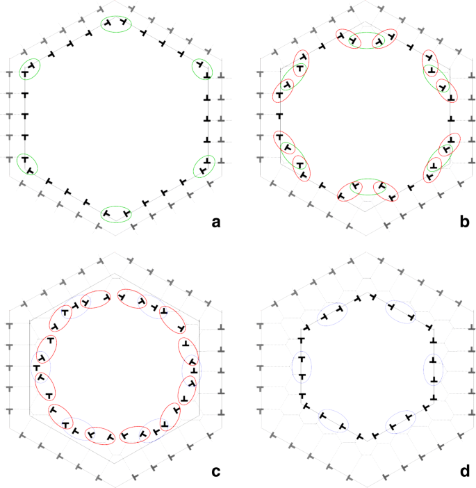

  

  Simplified model proposed to explain the boundary migration by progressive cellular rings: a) simple glide of dislocations; b) an unstable situation is reached at the corners when dislocations with Burgers vectors rotated by 60^∘ approach one to the other and proceed to an effective climb mechanism. Pairs of dislocations that undergo this climb process are highlighted by green circles just before -in a)- and just after -in b)- the climb process; c) the dislocations at the corners propagate along the sides by a chain of effective climb events, see red circles in b) and corresponding red circles in c); d) a cellular hexagonal-shaped ring is closed and the dislocation number per side is lowered through a three-to-two annihilation reaction, see blue circles in c) and d)

• the effective climb of the dislocations meeting at the six corners (see green circles in Fig. 10a-b;

• subsequent propagation of effective climb along each side of the hexagon (see red circles in Fig. 10b-c;

• after propagation, a first hexagonal shaped ring is closed by partial annihilation between two or more dislocations (see for example the blue circles in Fig. 10c and d.

In brief, the grain collapse proceeds through a succession of dislocation glide perpendicularly to the hexagonal facets, propagation of climb events along the facets and one annihilation event per facet. The overall effect of this mechanism is an increase of the misorientation angle θ together with the decrease of the grain area.

The link between the misorientation angle θ and grain area A may be identified as follows. As explained above, the process is analyzed as the successive formation of hexagons. We label the hexagons by the index n. At stage n, we note l_n, R_n, θ_n, $N_{n}^{side}$ and d_n the length of the facets, the distance of the facets from the centre of the hexagon, the misorientation angle, the number of dislocations along each facet and the average distance between dislocations, respectively. Using Frank’s formula (Frank 1950), we have:

$$d_{n} = \frac{\parallel \mathbf{b} \parallel}{2\sin (\theta_{n}/2)} \sim \frac{\parallel \mathbf{b} \parallel}{\theta_{n}}, $$

The facet length l_n and the distance R_n are geometrically linked (see Fig. 9-b):

$$l_{n} = \frac{2}{\sqrt{3}}R_{n}, $$

and d_n is defined by:

$$d_{n} = \frac{l_{n}}{N_{n}^{side}}. $$

Now, we analyze the transition from hexagon n to hexagon (n+1) as follows:

• first, all the dislocations that sit along the facets glide perpendicularly to the facets, and their number remains constant. Under the hypothesis that the distance between two neighboring dislocations that are separated by a corner is equal to the average distance, a simple geometrical analysis shows that an unstable situation (i.e., two dislocations come close to each other) is reached after a gliding equal to d_n;

• then, the effective climb events start at the corners, propagate along the boundary and stop when the new hexagon is closed through one annihilation event per side.

This kinematics is associated with the following recursive relations:

$$\begin{array}{*{20}l}& R_{n+1} = R_{n} - d_{n}, \\ & N^{side}_{n+1} = N_{n}^{side} - 1, \\ & d_{n+1} = \frac{2}{\sqrt{3}} \frac{R_{n+1}}{N^{side}_{n+1}}. \end{array} $$

It is straightforward to integrate recursively these relations and to calculate, for each index n, the actual value of the misorientation angle θ_n and hexagon area A_n:

$$\begin{array}{*{20}l} & \theta_{n} = 2 \sin^{-1} \left(\frac{\parallel \mathbf{b} \parallel}{2 d_{n}} \right), \\ & A_{n} = 2\sqrt{3} R_{n}^{2}. \end{array} $$

We used this kinematics to estimate the co-evolution of the misorientation θ and grain area A for a grain with initial misorientations θ₀=10^∘ and θ₀=15^∘, area $A_{0} = 2\sqrt {3}R_{0}^{2}$ with R₀=44.74σ. The result is shown in Fig. 11 where, for comparison, we also report the result obtained by the atomistic simulations. First, we observe that the model reproduces the grain rotation. This means that a coupled normal-tangential motion of grain boundary is embedded in the local mechanisms at the root of our model (glide, effective climb, annihilation). Second, we observe that our approximate hexagonal kinematics reproduces the atomistic simulation qualitatively, even if a quantitative agreement is not obtained, which is not surprising, taking into account the simplicity of the geometrical model we have proposed.

Fig. 11

Evolution of the misorientation θ as a function of the grain size predicted by the toy model (in red) compared with the results obtained by atomistic simulations (in blue) for θ₀=10^∘ (left) and for θ₀=15^∘ (right)

That being said, we think that the overall agreement between the simulation and the simple model confirms the validity of the local mechanisms (glide, effective climb, and three-to-two annihilation processes) that we identified as being at the origin of the grain shrinking mechanism for small initial misorientation. These mechanisms generate grain rotation (more precisely, an increase in the misorientation) in agreement with the atomistic simulations, thereby confirming the existence of a coupled motion. Finally, it is worth mentioning that the change of misorientation angle towards higher values that we observe here when the initial misorientation is low (θ₀<15^∘), is also in agreement with the predictions of the variational model proposed in ref. (Cahn and Taylor 2004).

Migration mechanism for high angle grain boundaries

When the initial misorientation is high (θ₀>15^∘), dislocations are no more identifiable at the GB since the spacing between 5-7 pairs resulting from the Delaunay triangulation is too small. As shown in Fig. 12, the GB can, however, be described by structural units. These units can be composed of a single 5-7 pair of defects or more. Their migration is no longer describable in terms of dislocation dynamics but can be explained by considering the local atomic position readjustments, which lead to the transformation from one lattice orientation to the other (Cahn et al. 2006a).

Fig. 12

Structure of a high angle grain boundary described in terms of structural units for θ₀=21.8^∘. Red and blue atoms have 5 and 7 NN, respectively

In Fig. 13a, we report the evolution of the misorientation angle for θ₀ ranging from 13.2^∘ to 27.8^∘. In all cases, the coupling effect (resulting in a change in θ) is present, except for θ₀=21.8^∘. We also stress that, in our simulations, the rotation direction of the grain (i.e., the sign of coupling) is opposite for θ₀<21.8^∘ and 21.8^∘<θ₀<30^∘. The fact that there is no coupling effect for some particular initial misorientations was already mentioned in the previous works (Trautt and Mishin 2012; Upmanyu et al. 2006). The absence of coupling for θ₀=21.8^∘ is justified by the fact that this misorientation corresponds to a CSL condition for the hexagonal grid (Σ7). However, this justification is incomplete because, as we can see from Fig. 13a, a non-zero coupling is clearly observed for the misorientation values 27.8^∘(Σ13) and 13.2^∘(Σ19), which also correspond to CSL conditions.

Fig. 13

a Misorientation as a function of the grain area (in σ² units) for several initial misorientation θ₀; b 5-7 pairs density $\protect \phantom {\dot {i}\!}\rho _{5-7}/\rho _{{5-7}_{0}}$ along the grain boundary (red curve) and change in the misorientation angle θ/θ₀ (blue curve) during grain shrinkage for the initial misorientations θ₀=21.8^∘

In this section, we analyze the atomistic mechanisms at the origin of the GB migration for the value θ₀=21.8^∘. As previously done with dislocations in the low misorientation case, we computed the density of 5-7 defects accommodating the misfit between the matrix and the grain during its shrinkage. The evolutions of the normalized quantities ρ_D(t)/ρ_D(t=0) and (θ(t)−θ₀)/θ₀ are reported in Fig. 13b. We observe that the density of 5-7 defects remains approximately constant during the grain shrinkage, although some fluctuations of the order of 5% are present. Therefore, as in the low misorientation case, we observe that the rotation of the grain is linearly related to the density of 5-7 defects along the boundary.

In order to clarify the kinematics observed for θ₀=21.8^∘ we kept track of the neighborhood of each atom during the grain shrinkage. We observed that there is a set of atoms that hardly move and whose first neighbor shell remains unchanged, even though the atoms within these shells are displaced. The positions of these “fixed” atoms, shown in Fig. 14a, are not random but are locally on a Σ7 coincidence sites grid. More precisely, several regions where a Σ7 coincidence sites lattice (CSL) grid can be observed, with transition zones between them. This is linked to the fact that seven different CSL grids can be defined for a Σ7 grain boundary, the different grids being related by a translation. All the above observations suggest that, for the special case of θ₀=21.8^∘, the migration of the boundary occurs by local adjustment of atoms rotating around these “fixed” positions.

Fig. 14

Atomic structure after the grain shrinkage (θ₀=21.8^∘): a atoms that have not changed their first nearest neighbors shell are represented in green; b atoms are colored according to the value of the $D^{(n)^{2}}$ coefficient (see text for details)

To better quantify this peculiar behavior, described above we propose the following calculation. We consider the relative position Δr_nm between the atom n and its first neighbor m at time t=0 and at time t^∗ after the GB passage. Then, following the approach proposed in Falk and Langer (1998), we try to identify a local linear transformation F⁽ⁿ⁾ that describes the atomic movements around the atom n. In order to do this, we minimize the mean-square difference between Δr_nm(t^∗) and the local displacement that would result from the action of F⁽ⁿ⁾ on Δr_nm(0), m=1,…,6:

$$ D^{(n)^{2}} = \sum_{m=1}^{6} \lVert \Delta \mathbf{r}_{nm}(t^{*}) - \mathbf{F}^{(n)}\Delta \mathbf{r}_{nm}(0)\lVert^{2}. $$

(17)

Numerically, the matrix F⁽ⁿ⁾ which minimizes $D^{(n)^{2}}$ is given by:

$$\begin{array}{*{20}l} \left(Y^{(n)}\right)_{ij}& = \sum_{m=1}^{6} (\Delta \mathbf{r}_{nm}(0))_{i}(\Delta \mathbf{r}_{nm}(0))_{j},\\ \left(X^{(n)}\right)_{ij} &= \sum_{m=1}^{6} (\Delta \mathbf{r}_{nm}(t^{*}))_{i} (\Delta \mathbf{r}_{nm}(0))_{j}, \end{array} $$

(18)

$$\begin{array}{*{20}l} \left(F^{(n)}\right)_{ij} &= \left(X^{(n)}\right)_{ik}\left(Y^{(n)}\right)_{kj}^{-1}. \end{array} $$

(19)

If, for a given atom n, this minimization process leads to a small enough $D^{(n)^{2}}$ (typically $D^{(n)^{2}} < 0.1$) then we may interpret the dynamics around the atom n as a uniform transformation associated with the local deformation gradient F⁽ⁿ⁾,:

$$ \Delta \mathbf{r}_{nm}(t^{*})\approx \mathbf{F}^{(n)} \Delta \mathbf{r}_{nm}(0). $$

(20)

Conversely, if the minimization does not lead to a small $D^{(n)^{2}}$, atomic movements around an atom n cannot be described by a local transformation matrix. The results of this overall procedure are reported in Fig. 14b, where we can see that the deviation $D^{(n)^{2}}$ is almost zero for atoms that sit on the coincidence sites while it takes higher values for the surrounding atoms. Furthermore, for the atoms inside the initial grain and for which $D^{(n)^{2}}<0.1$, we have analyzed the deformation gradient F⁽ⁿ⁾. The histogram of the four components of F⁽ⁿ⁾ are presented in Fig. 15. From these histograms, we conclude that the deformation gradient at the vicinity of the atoms considered is found to be

$$ \mathbf{\overline{F}}=\left(\begin{array}{lc} 0.9320 & -0.3738 \\ 0.3735 & 0.9291\\ \end{array}\right), $$

(21)

Fig. 15

Histogram of the deformation gradients inside the grain for atoms such that $D^{(n)^{2}}<0.1$ after the grain shrinkage (θ₀=21.8^∘)

with a standard deviation smaller than 1.5×10⁻³ on each component. Because the standard deviations are small, $\mathbf {\overline {F}}$ can reasonably be thought as representative of the local deformation gradient F⁽ⁿ⁾. Obviously, $\mathbf {\overline F}$ is anti symmetric. As its determinant is close to 1 $(\det \mathbf {\overline {F}} \approx 1)$, we conclude that $\mathbf {\overline {F}}$ describes a rotation. In conclusion, the movements of atoms surrounding the ones sitting on the coincidence sites positions can be interpreted as rigid rotation. The associated rotation angle is found to be $\theta \approx \sin ^{-1}(\overline {F}_{21}) = 21.9^{\circ }$, which is approximately the value of the misorientation angle.

The local rotation in the neighborhood of atoms located on the Σ7 coincidence site lattices can also be described in terms of the dynamics of 5-7 defects (Fig. 16). These 5-7 defects (blue-red atom pairs), located at the grain boundary, migrate in between the coincidence lattice sites atoms (black atoms), the latter keeping their 6 NN. The evolution of the orientation of the 5-7 defects during their migration reveals that their migration cannot be described as a glide mechanism (a video is available as a supplementary material).

Fig. 16

a-d 5-7 defects walk during grain shrinkage for θ₀=21.8^∘. Atoms on the Σ7 coincidence site lattice are shown in black, the coincidence sites grid in dotted line

Summary, conclusion and perspectives

In the present work, a stochastic dynamics for the atomistic modeling of crystalline materials is presented and tested in the context of GB migration. Atoms motion is described through an overdamped Langevin formalism in order to avoid crystal vibrations that limit the time-step size to be used in the integration of equations. The convergence of the dynamics to the correct equilibrium in the canonical ensemble is demonstrated. The model is extended to simulate the (NPT) ensemble by adding 9 DOF which describe the macroscopic deformation gradient of the simulation box. Convergence to the correct equilibrium distribution for the system of (N+9) DOF is guaranteed as well. A possible justification for applying the proposed overdamped dynamics to crystalline materials is suggested by numerical calculations of the autocorrelation functions of atoms position and velocities. Finally, a first numerical application of the proposed model is performed in the field of GB migration. For this application, we focused on a simple case study where GB motion is driven only by curvature and temperature, and we simulated the shrinking of a circular island grain embedded in a monocrystalline matrix. In order to validate the model, we compared our results with the ones obtained from MD simulations. The good agreement between the two methodologies confirms the applicability of the overdamped Langevin dynamics for modeling the microstructural evolutions in crystalline materials. Furthermore, we highlight interesting characteristics of the mechanisms driving the GB migration in the low and high misorientation cases. For low angle GB, we observed that the GB migration proceeds by a combination of dislocation glide, effective climb, and annihilation reaction. A geometrical model is proposed to explain these particular migration mechanisms. The change in the misorientation θ predicted by this “simple model” shows an overall agreement with those obtained by simulations. For high misorientation GB, we verified that the existence or absence of the coupled motion, highlighted in previous works, is strictly linked to the GB structure. We verified that for misorientations corresponding to the CSL Σ7, atoms on coincidence sites act as “fixed points” thus prevent any rotation of the grain. The boundary migration proceeds by local rotations of atomic positions around these points.

The overdamped approach proposed here is of course fully 3D and a 3D analysis of a phase transition using a many-body interatomic potential is in progress and will be submitted for publication shortly (Baruffi 2018).

In conclusion, the overdamped LD seems to be a suitable instrument for the atomistic modeling of crystalline materials. Future perspectives are: (i) the application of the overdamped LD for the study of other physical phenomena involving the microstructural evolution in metallic alloys (for example phase transitions) and, (ii) most importantly, the derivation of Langevin equations through an explicit coarse graining of the Newtonian dynamics, the anticipated outcome of this procedure being a coarse-grained potential and the associated overdamped dynamics.

Appendix

We consider a stochastic equation with white noise for the set of positions $\{ x_{i}^{n}\}$ of the form:

$$ \mathrm{d}x_{i}^{n}(t) = f_{i}^{n}(\{ x_{i}^{n}(t)\}) \mathrm{d}t + B \mathrm{d}W_{i}^{n}(t), $$

(22)

where $f_{i}^{n}$ is the ith component of the force on atom n derived from the interaction energy ϕ as $f_{i}^{n}\left (\left \{x_{i}^{n}(t)\right \}\right) = - \frac {\partial \Phi }{\partial x_{i}^{n}}$ and the differential dW(t) denotes an infinitesimal increment of the Wiener process $W_{i}^{n}(t)$ and $B=\sqrt {2 \nu k_{B} T}$ to enforce the correct equilibrium properties discussed in the text. The integral form of Eq. (22) is given by

$$ x_{i}^{n}(t) = \int_{t_{0}}^{t}f_{i}^{n}\left(\left\{x_{i}^{n}(t^{\prime})\right\}\right) \mathrm{d}t^{\prime} + \int_{t_{0}}^{t} B\mathrm{d}W_{i}^{n}(t^{\prime}) + x_{i}^{n}(t_{0}), $$

(23)

where the first term in the rhs. is a Riemann integral and the second term is a stochastic integral. To numerically evaluate Eq. (23) we implement an explicit predictor-corrector method which results in the following numerical scheme:

$$ \begin{aligned} x_{i}^{n}(t + \Delta t) &= x_{i}^{n}(t) + {\frac{1}{2}}\left[f_{i}^{n}\left(\left\{\bar x_{i}^{n}(t+\Delta t)\right\}\right)+ f_{i}^{n}(\{x_{i}^{n}(t)\})\right] \Delta t +B \Delta W_{i}^{n}(t),\\ \bar x_{i}^{n}(t + \Delta t)&= x_{i}^{n}(t) +f_{i}^{n}\left(\left\{x_{i}^{n}(t)\right\}\right) \Delta t + B\Delta W_{i}^{n}(t), \end{aligned} $$

(24)

where the finite increment $\Delta W_{i}^{n}(t) = W_{i}(t + \Delta t) - W_{i}^{n}(t)$ can be calculated as $\Delta W_{i}^{n}(t) = \sqrt {\Delta t} \xi (t), \Delta t \in \mathbb {R}$ and ξ(t) taken from a normal distribution with unit variance. In the numerical simulations we used a time-step Δt=2×10⁻³.

References

T. Ando, T. Meguro, I. Yamato, Multiple time step brownian dynamics for long time simulation of biomolecules. Mol. Simul.29(8), 471–478 (2003).
A. Ask, S. Forest, B. Appolaire, K. Ammar, O. U. Salman, A cosserat crystal plasticity and phase field theory for grain boundary migration. J. Mech. Phys. Solids. 115:, 167–194 (2018).
D. W. Bainbridge, H. L. Choh, E. H. Edwards, Recent observations on the motion of small angle dislocation boundaries. Acta Metall.2(2), 322–333 (1954).
L. A. Barrales-Mora, J. -E. Brandenburg, D. A. Molodov, Impact of grain boundary character on grain rotation. Acta Mater.80:, 141–148 (2014).
L. A. Barrales-Mora, D. A. Molodov, Capillarity-driven shrinkage of grains with tilt and mixed boundaries studied by molecular dynamics. Acta Mater.120:, 179–188 (2016).
C. Baruffi, Application of an overdamped langevin dynamics to the study of microstructural evolutions in crystalline materials. PhD thesis manuscript, Université Paris-Sorbonne (2018).
L. K. Béland, P. Brommer, F. El-Mellouhi, J. -F. Joly, N. Mousseau, Kinetic activation-relaxation technique. Phys. Rev. E Stat. Nonlin. Soft Matter Phys.84(4 Pt 2), 046704 (2011).
B. Béucia, P. Franciosi, S. Queyreau, D. Chaubet, B. Bacroix, in IOP Conference Series: Materials Science and Engineering, vol. 89. TEM observations of grain boundary mobility under thermal and plasticity effects (IOP Publishing Ltd.Bristol, 2015), p. 012019.
A. B. Bortz, M. H. Kalos, J. L. Lebowitz, A new algorithm for monte carlo simulation of ising spin systems. J. Comput. Phys.17(1), 10–18 (1975).
J. -E. Brandenburg, L. Barrales-Mora, D. Molodov, On migration and faceting of low-angle grain boundaries: Experimental and computational study. Acta Mater.77:, 294–309 (2014).
V. Bulatov, F. F. Abraham, L. Kubin, B. Devincre, S. Yip, Connecting atomistic and mesoscale simulations of crystal plasticity. Nature. 391(6668), 669–672 (1998).
J. W. Cahn, Y. Mishin, Recrystallization initiated by low-temperature grain boundary motion coupled to stress. Int. J. Mater. Res.100(4), 510–515 (2009).
J. W. Cahn, Y. Mishin, A. Suzuki, Coupling grain boundary motion to shear deformation. Acta Mater.54(19), 4953–4975 (2006a).
J. W. Cahn, Y. Mishin, A. Suzuki, Duality of dislocation content of grain boundaries. Phil. Mag.86(25-26), 3965–3980 (2006b).
J. W. Cahn, J. E. Taylor, A unified approach to motion of grain boundaries, relative tangential translation along grain boundaries, and grain rotation. Acta Mater.52(16), 4887–4898 (2004).
B. Chen, K. Lutker, J. Lei, J. Yan, S. Yang, H. -k. Mao, Detecting grain rotation at the nanoscale. Proc. Natl. Acad. Sci.111(9), 3350–3353 (2014).
K. R. Elder, M. Katakowski, M. Haataja, M. Grant, Modeling elasticity in crystal growth. Phys. Rev. Lett.88(24), 245701 (2002).
F. El-Mellouhi, N. Mousseau, L. J. Lewis, Kinetic activation-relaxation technique: An off-lattice self-learning kinetic monte carlo algorithm. Phys. Rev. B. Condens. Matter. 78(15), 153202 (2008).
M. L. Falk, J. S. Langer, Dynamics of viscoplastic deformation in amorphous solids. Phys. Rev. E. 57(6), 7192 (1998).
D. Farkas, A. Frøseth, H. Van Swygenhoven, Grain boundary migration during room temperature deformation of nanocrystalline ni. Scr. Mater.55(8), 695–698 (2006).
FC Frank, Report of the symposium on the plastic deformation of crystalline solids, eds. Mellon Institute of Industrial Research, Carnegie Institute of Technology and Office of Naval Research; publisher U.S. Government Printing Office (Mellon Institute, Pittsburgh, 1950).
A. Finel, Y. Le Bouar, B. Dabas, B. Appolaire, Y. Yamada, T. Mohri, Sharp phase field method. Phys. Rev. Lett.121:, 025501 (2018).
A. Finel, Y. Le Bouar, A. Gaubert, U. Salman, Phase field methods: Microstructures, mechanical properties and complexity. C. R. Phys.11:, 245–256 (2010).
P. -A. Geslin, B. Appolaire, A. Finel, Investigation of coherency loss by prismatic punching with a nonlinear elastic model. Acta Mater.71:, 80–88 (2014).
D. Gianola, S. Van Petegem, M. Legros, S. Brandstetter, H. Van Swygenhoven, K. Hemker, Stress-assisted discontinuous grain growth and its effect on the deformation behavior of nanocrystalline aluminum thin films. Acta Mater.54(8), 2253–2263 (2006).
G. Gottstein, L. Shvindlerman, On the orientation dependence of grain boundary migration. Scr. Metall. Mater.27(11), 1515–1520 (1992).
G. Gottstein, L. S. Shvindlerman, Grain Boundary Migration in Metals | Thermodynamics, Kinetics, Applications, Second Edition (Taylor & Francis, Boca Raton, 2009).
E. R. Homer, S. M. Foiles, E. A. Holm, D. L. Olmsted, Phenomenology of shear-coupled grain boundary motion in symmetric tilt and general grain boundaries. Acta Mater.61(4), 1048–1060 (2013).
W. G. Hoover, Constant-pressure equations of motion. Phys. Rev. A. 34(3), 2499 (1986).
Y. Huang, F. Humphreys, Measurements of grain boundary mobility during recrystallization of a single-phase aluminium alloy. Acta Mater.47(7), 2259–2268 (1999).
R. Kobayashi, J. A. Warren, W. C. Carter, A continuum model of grain boundaries. Physica D: Nonlinear Phenom.140(1), 141–150 (2000).
A. Laio, M. Parrinello, Escaping free-energy minima. Proc. Natl. Acad. Sci. U. S. A.99(20), 12562–12566 (2002).
C. H. Li, E. H. Edwards, J. Washburn, E. R. Parker, Stress-induced movement of crystal boundaries. Acta Metall.1(2), 223–229 (1953).
M. Legros, D. S. Gianola, K. J. Hemker, In situ TEM observations of fast grain-boundary motion in stressed nanocrystalline aluminum films. Acta Mater.56(14), 3380–3393 (2008).
L. Ma, X. Li, C. Liu, From generalized langevin equations to brownian dynamics and embedded brownian dynamics. J. Chem. Phys.145(11), 114102 (2016a).
L. Ma, X. Li, C. Liu, The derivation and approximation of coarse-grained dynamics from langevin dynamics. J. Chem. Phys.145(20), 204117 (2016b).
M. Manghi, X. Schlagberger, Y. -W. Kim, R. R. Netz, Hydrodynamic effects in driven soft matter. Soft Matter. 2:, 653–668 (2006).
A. Minami, A. Onuki, Nonlinear elasticity theory of dislocation formation and composition change in binary alloys in three dimensions. Acta Mater.55(7), 2375–2384 (2007).
Y. Mishin, M. Asta, J. Li, Atomistic modeling of interfaces and their impact on microstructure and properties. Acta Mater.58(4), 1117–1151 (2010).
D. A. Molodov, T. Gorkaya, G. Gottstein, in Materials Science Forum, vol. 558. Mechanically driven migration of <100> tilt grain boundaries in Al-bicrystals (Trans Tech PublicationsSwitzerland, 2007), pp. 927–932.
D. A. Molodov, T. Gorkaya, G. Gottstein, Dynamics of grain boundaries under applied mechanical stress. J. Mater. Sci.46(12), 4318–4326 (2011).
F. Mompiou, D. Caillard, M. Legros, Grain boundary shear–migration coupling—i. in situ tem straining experiments in al polycrystals. Acta Mater.57(7), 2198–2209 (2009).
E. Nelson, Dynamical Theories of Brownian Motion (Princeton University Press; Second edition, Princeton University, 1967).
S. Nosé, A molecular dynamics method for simulations in the canonical ensemble. Mol. Phys.52(2), 255–268 (1984).
W. B. Paul, Molecular dynamics simulation, elementary methods. Adv. Mater.5(3), 223–224 (1993).
S. Plimpton, Fast parallel algorithms for Short-Range molecular dynamics. J. Comput. Phys.117(1), 1–19 (1995).
T. Pusztai, G. Bortel, L. Gránásy, Phase field theory of polycrystalline solidification in three dimensions. Europhys. Lett.71(1), 131–137 (2005).
T. Radetic, C. Ophus, D. Olmsted, M. Asta, U. Dahmen, Mechanism and dynamics of shrinking island grains in mazed bicrystal thin films of au. Acta Mater.60(20), 7051–7063 (2012).
A. Rahman, Correlations in the motion of atoms in liquid argon. Phys. Rev.136(2A), 405 (1964).
T. Rupert, D. Gianola, Y. Gan, K. Hemker, Experimental observations of stress-driven grain boundary migration. Science. 326(5960), 1686–1690 (2009).
O. U. Salman, A. Finel, R. Delville, D. Schryvers, The role of phase compatibility in martensite. J. Appl. Phys.111(10), 103517 (2012).
O. U. Salman, B. Muite, A. Finel, Origin of stabilization of macrotwin boundaries in martensites. Eur. Phys. J. B. 92(1), 20 (2019).
O. U. Salman, L. Truskinovsky, Minimal integer automaton behind crystal plasticity. Phys. Rev. Lett.106(17), 175503 (2011).
Z. W. Shan, R. K. Mishra, S. A. Syed Asif, O. L. Warren, A. M. Minor, Mechanical annealing and source-limited deformation in submicrometre-diameter ni crystals. Nat. Mater.7(2), 115–119 (2008).
Z. Trautt, A. Adland, A. Karma, Y. Mishin, Coupled motion of asymmetrical tilt grain boundaries: Molecular dynamics and phase field crystal simulations. Acta Mater.60(19), 6528–6546 (2012).
Z. Trautt, Y. Mishin, Grain boundary migration and grain rotation studied by molecular dynamics. Acta Mater.60(5), 2407–2424 (2012).
Z. Trautt, Y. Mishin, Capillary-driven grain boundary motion and grain rotation in a tricrystal: a molecular dynamics study. Acta Mater.65:, 19–31 (2014).
M. Upmanyu, D. J. Srolovitz, A. Lobkovsky, J. A. Warren, W. Carter, Simultaneous grain boundary migration and grain rotation. Acta Mater.54(7), 1707–1719 (2006).
A. F. Voter, Hyperdynamics: Accelerated molecular dynamics of infrequent events. Phys. Rev. Lett.78(20), 3908–3911 (1997).
A. Vuppuluri, S. Vedantam, Grain growth rate for coupled grain boundary migration and grain rotation in nanocrystalline materials. Philos. Mag. Lett.96(9), 339–346 (2016).
L. Wang, J. Teng, P. Liu, A. Hirata, E. Ma, Z. Zhang, M. Chen, X. Han, Grain rotation mediated by grain boundary dislocations in nanocrystalline platinum. Nat. Commun.5:, 4402 (2014).
M. Winning, G. Gottstein, L. Shvindlerman, Stress induced grain boundary motion. Acta materialia. 49(2), 211–219 (2001).
K. -A. Wu, P. W. Voorhees, Phase field crystal simulations of nanocrystalline grain growth in two dimensions. Acta Mater.60(1), 407–419 (2012).
S. Yip, Handbook of Materials Modeling, vol. 1 (Springer, Netherlands, 2005).
P. Zhang, O. U. Salman, J. -Y. Zhang, G. Liu, J. Weiss, L. Truskinovsky, J. Sun, Taming intermittent plasticity at small scales. Acta Mater.128:, 351–364 (2017).
L. A. Zepeda-Ruiz, A. Stukowski, T. Oppelstrup, V. V. Bulatov, Probing the limits of metal plasticity with molecular dynamics simulations. Nature. 550:, 492 (2017).
Acknowledgements
AF and YLB would like to thank to Saurav Aryan for his previous work during his master internship in LEM.
Funding
CB and BB gratefully acknowledge ANR (Agence Nationale de la Recherche), CGI (Commissariat à l’Investissement d’Avenir) for their financial support through Labex SEAM (Science and Engineering for Advanced Materials and devices), ANR 11 LABX 086, ANR 11 IDEX 05 02.
Availability of data and materials
The datasets used and/or analyzed during the current study are available from the corresponding author on reasonable request.
Author information
Authors and Affiliations
Contributions
All authors contributed to the writing of the article. AF and CB developed the model. CB, AF, OUS and YLB contributed to the development of the code. All authors contributed to the analysis of the numerical results, read and approved the final manuscript.
Corresponding author
Ethics declarations
Competing interests
The authors declare that they have no competing interests.
Publisher’s Note
Springer Nature remains neutral with regard to jurisdictional claims in published maps and institutional affiliations.
Rights and permissions
Open Access This article is distributed under the terms of the Creative Commons Attribution 4.0 International License (http://creativecommons.org/licenses/by/4.0/), which permits unrestricted use, distribution, and reproduction in any medium, provided you give appropriate credit to the original author(s) and the source, provide a link to the Creative Commons license, and indicate if changes were made.
About this article
Cite this article
Baruffi, C., Finel, A., Le Bouar, Y. et al. Overdamped langevin dynamics simulations of grain boundary motion. Mater Theory 3, 4 (2019). https://doi.org/10.1186/s41313-019-0016-1
Received:
Accepted:
Published:
DOI: https://doi.org/10.1186/s41313-019-0016-1